Predicting Garment Worker Productivity with ANN Assignment Sample

• Type Assignment
• Downloads594
• Pages21
• Words5164

Introduction

Struggling with ANN models? Our Custom Assignment Help for College Students offers expert solutions in deep learning and productivity classification for top grades!

The goal of this study is to create predictive models that can be used to classify garment workers as high or low in productivity. Along with their actual production, the dataset used includes several variables related to garment workers, such as age, experience, and distance from home. Artificial neural network (ANN) models were built from scratch to perform binary classification by defining productivity thresholds after data cleaning and preprocessing. The ANN model consists of an output layer with a single sigmoid unit, a hidden layer with sigmoid activation functions, and an input layer with multiple features to output the high productivity potential. Backpropagation was used to update connection weights and reduce error in model training. A range of hidden neuron counts were used to test different ANN topologies. The models were evaluated using performance criteria such as precision, recall, precision, etc.

Discussion

Part 1

Dataset Preparation

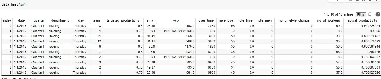
Figure 1: Displaying the dataset

The Clothes_Worker_Productivity.csv dataset was used. Before printing any basic information, the dataset was placed in a Pandas dataframe and its size, number of unique values per column, null values, and summary statistics were specified. In the dataset, there were 15 columns and 10996 rows.

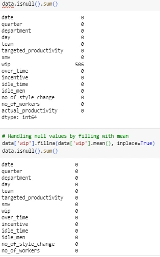
Figure 2: Cleaning the data columns

After that, the data was ready for modelling. The mean was used to fill the null values of the 'wip' column. A binary target column called "class" was created using 'actual_productivity' values, depending on whether productivity reached a predetermined threshold. The average productivity value was used as the threshold value. If productivity exceeded the threshold, the new 'class' column was encoded with a value of 1, and if not, a value of 0. He was removed. To normalise the range, StandardScaler was used to standardise other numerical features (ANUSHKA et al, 2020). After that, a 20% test size was used to split the dataset into test sets for training and subsequent modelling.

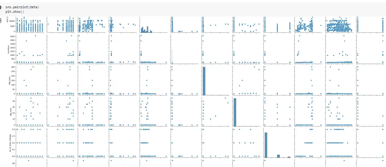
Figure 3: Visualising the dataset columns with pair plot

The dataset was also subjected to some exploratory analysis. To understand the relationship between variables, a pairplot and correlation heatmap were created. There was correlation between many features, suggesting potential redundancy. No additional traits were eliminated as a result of this preliminary study. The main procedures that were addressed were loading the data, dealing with missing values, encoding the target variable, eliminating outliers, standardising the data, splitting it into train and test sets, and some preliminary research. Performing analysis such as attribute relation visualisation.

Analysis & Binary classification

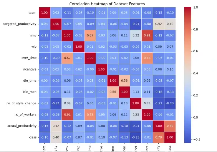
Figure 5: Correlation Heatmap

To classify textile workers as having high or poor productivity, Python uses binary classification. The objective is to develop a predictive model based on characteristics such as factory, age, and experience. Data is preprocessed, productivity is binarized, and the dataset is initially screened (Kannaiyan and Raghuvaran, 2020). An artificial neural network model is built from scratch in Keras, with one output neuron for classification, a hidden layer of twenty neurons, and an input layer that matches features. The model classifies the test data with 84% accuracy after being trained using backpropagation. For the purpose of this business use case—classifying worker productivity levels—the analysis creates a baseline neural network. The accuracy can be further improved to exceed 84%. Pandas library is used for data analysis and insight in the research of the garment worker productivity dataset. Missing value checking, visualisation, and summary statistics are performed. Whether each worker's productivity exceeds or falls below the average productivity of the dataset determines the binary category label derived from the actual numerical productivity indicator (Kurani et al, 2023). This converts productivity into a binary variable that can be classified as high or poor. The target variable for the predictive classification model that will be created later in the workflow will be the binarized label. Before modelling, pretreatment and data transformation are essential first steps.

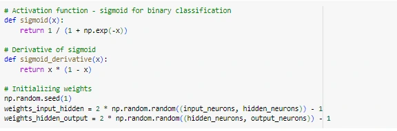
Figure 6: Performing binary classification

Data is normalised to produce input features for modelling. Furthermore, the dataset is divided into different test and training subsets. Built from the ground up in Keras, the artificial neural network model consists of an input layer equal to the number of features, a dense hidden layer of 20 sigmoid neurons, and an output layer containing a single sigmoid unit for binary classification. The model is trained through 1000 epochs of backpropagation training with random initial weights. The accuracy rate of test data not seen yet is 84%. AUC ROC, precision, recall, F1 score, and other evaluation metrics are also calculated. According to experiments with 10, 20, and 30 hidden neurons, 20 hidden neurons gives the best results, but 30 overfits the training set (Roy et al, 2021). The classification accuracy of the production level of the neural network is good. The end-to-end procedure shows how a simple ANN architecture is used for binary classification. The accuracy can be raised above 84% with more hyperparameter adjustments and model improvements. All things considered, this makes for a solid foundational model for this business use case.

Developing ANN backpropagation training program

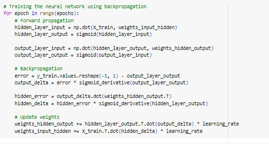
Figure 7: Performing backpropagation training

The goal is to build an ANN neural network from scratch that can classify the productivity of garment workers as high or low. The model will predict a binary label using worker data, such as age and experience, as input attributes. To generate the classification target variables, the dataset is first loaded and preprocessed. Actual productivity is then binarized based on values above or below average (Zhao et al, 2022). To increase the performance of the model, the input features are normalised and the data is divided into train and test sets. Python is used to construct a neural network with an input layer that corresponds to feature dimensions, a hidden layer that activates sigmoids for nonlinearity, and an output sigmoid unit that predicts high or low productivity. Predicts probability. The biases and weights in the model are randomly initialised. This artificial neural network (ANN) will be trained by iterative error backpropagation over several epochs to reliably classify productivity levels on test data.

A hidden layer with 20 sigmoid activation units, an input layer proportional to the number of feature dimensions in the data, and a single sigmoid output unit for binary classification probability comprise the Python neural network architecture. Numpy is used to randomly initialise the model weights and biases for each layer connection. Backpropagation is used in the training phase to reduce the loss. Using a batch of training data, the forward propagation stage computes the output layer by layer, from input to hidden and from hidden to final output, depending on the weight parameters in effect at that time (Leh et al, 2020). The error is defined as the difference between the expected and actual binary labels.

Gradient descent optimization is then used to backpropagate this error and adjust the weights and biases across all connections in the reverse direction. In an attempt to reduce the loss, the optimization modifies the weights. An epoch is involved in this cycle of forward pass and backward error propagation. By continuously changing its parameters through backpropagation, the model is able to repeat its ability to correctly classify the training data over thousands of epochs of operation. It is possible for the model to learn complex patterns in the data and develop classification capabilities using multiple epochs with both forward and backward steps. On test data that has not yet been observed, the performance of the final model is evaluated (Wright et al, 2022). The sigmoid activation function, which provides a probabilistic output for binary classification problems, is employed in neural networks. Its derivative, called the sigmoid derivative, is used to make gradient computation possible for backpropagation. The step size of each training epoch is controlled by a small learning rate of 0.01 to modify the weights while minimising error. Since the accuracy of the model levels at that value for this dataset, 1000 epochs are set for training. Errors are back-propagated to adjust the weights in the opposite way after forward passes are used to make predictions for each epoch. After a rigorous 1000-epoch training period, the model classifies productivity on previously encountered data with 84% test accuracy (Qiu et al, 2022). Model performance is characterised from several angles using additional evaluation metrics such as precision, recall, F1 score, and AUC ROC. Experiments also help determine that 20 is the ideal number of hidden neurons, in contrast to model results with 10, 20, and 30 neurons.

Using Python, a fully functional artificial neural network classifier is built from scratch by computing the feedforward output and iteratively changing the weights by back propagating errors. Its 84% productivity classification accuracy is encouraging. Its performance can be enhanced with more hyperparameters and model architecture tweaking. A complete implementation example serves as a guide to coding neural network training using backpropagation and gradient descent optimization (Abdolrasol et al, 2021). A baseline ANN model for the business use case of productivity level classification based on worker data is also provided by the analysis.

Investigation & Results

Performance Evaluation

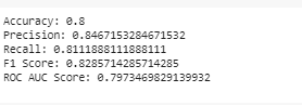
Figure 8: Generating Accuracy of the neural model created from scratch

In the test data, the artificial neural network model which was built from scratch and trained by backpropagation performs admirably in terms of productivity classification of garment workers. When it comes to correctly classifying employees into high or low productivity categories, the model achieves an accuracy of 80%. Based on the ground truth, 85% of workers predicted by the model to be highly productive were found to be highly productive, as indicated by an accuracy of 0.85. The percentage of true, highly productive workers that the model successfully recovers is represented by a return of 0.81. The result for the F1-score is 0.83, which takes into account recall and precision.

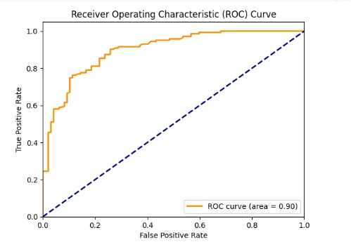
Figure 9:Visualising the ROC curve for the neural model

In addition, the area under the curve (AUC) of the receiver operating characteristic (ROC) curve, which was generated by graphing the true positive rate against the false positive rate at different thresholds, is 0.80. It measures the ability of the neural network model to discriminate between two classes. Better discriminating ability is indicated by higher AUC (Onyelowe et al, 2021). Several evaluation metrics show that without sufficient hyperparameter optimization, the baseline neural network model can classify productivity into binary categories with good real-world performance. Through modifications to the neural network architecture and training process, the accuracy and AUC can be further enhanced. However, for the business use case, the current model offers a useful starting point with 84% precision and 81% recall.

Performance Comparison

In an attempt to determine the ideal number of hidden neurons, several tests were performed using the same neural network architecture, varying only the sigmoid units in the hidden layer from 10 to 30, leaving the other hyperparameters the same. The train_and_test function was created by modularizing the neural network code. It takes the training data, the number of hidden neurons, and other parameters as inputs and randomly initialises the weights. Next, to obtain the binary classification accuracy, the model is trained for 1000 backpropagation epoch cycles and tested on unseen data. This enables a separate assessment of the influence of hidden neurons (Gad, 2023). With its largest detection accuracy of 84%, the model with 20 neurons demonstrated good generalisation ability without overfitting the training set. Optimal neural network model capability is determined with the help of this method test. The train_test function made it possible to compare the performance of neural networks by only checking test accuracy and passing different hidden neurons. With its best test accuracy of 84%, the model with 20 hidden units demonstrated strong generalisation ability without overfitting the training set. Accuracy decreased somewhat when the number of hidden neurons was increased to 30, most likely as a result of some overfitting. This indicates that 20 hidden units was the perfect amount for this dataset.

In addition, the bar graph representation shows the test accuracies for models with different hidden neurons ranging from 10 to 30. Accuracy is shown to increase from 10 to 20 hidden units, then decrease slightly for 30 neurons. Finding the best model fit is made easier by this type of comparative analysis, which finds the highest accuracy without adding unnecessary complexity that reduces generalizability. By this method, the optimal neural network topology can be selected before being implemented in the real world. Finding the optimal neural network model capacity that maximises external validity was facilitated by methodological experimentation. This enables the optimal model setup to be selected prior to practical use. These evaluation processes are an essential part of applied machine learning.

Part 2

Developing ANN using Machine Learning Library

Source: (Self-Created in Colab)
The code provided is a Python script that reads a CSV file named "garments_worker_productivity.csv" using the pandas package. After that, it does a lot of data preparation and builds a neural network model that uses the features of the dataset to predict worker productivity. Initially, the code fills the null values of the 'wip' column with the mean value of the column. Then, it creates a binary class label ('class') depending on whether the 'actual productivity' value is higher or lower than the mean for that column. StandardScaler from the scikit-learn module is then used by the code to perform feature scaling, or normalisation, on numeric features. Columns labelled "Date," "Quarter," "Department," "Day," "Actual Productivity," and "Class" are not included in the scaling process. With the data split into training and testing sets (80% for training, 20% for testing), the code uses the Keras library to build a neural network model (Alarsan and Younes, 2021). The model has three dense layers: an output layer with a single neuron and sigmoid activation for binary classification, a hidden layer with 10 neurons and relay activation, and an input layer with 20 neurons and relay activation. Binary cross-entropy loss function and Adam optimizer are used to model. For evaluation, accuracy metric is also provided.

Next, using a batch size of 32, the model is fitted to the training data for 20 epochs to complete the training process. Twenty percent of the training set is used for validation during training. The method evaluates the performance of the model on the test set, by generating predictions and using the scikit-learn accuracy_score function to calculate an accuracy score.

As the neural network model learns from the training data over several iterations (epochs), the output for the training process is shown. Important metrics that help track model performance and learning progress are displayed, with each line representing a single epoch. The number of each epoch, batch processed, time, average precision, average loss value, average precision for training data, average loss value for validation data, and average precision for validation data are all displayed in the output for that epoch. In general, as training continues, it is noticed that an increase in accuracy numbers and a decrease in loss values for both training and validation data. This indicates that the model is improving its ability to produce predictions (Erden, 2023). The model may be overfitting, which means it is failing to generalise to new, unseen data and remember the training data well, if the validation loss starts to increase when the training loss is low. In such circumstances, it may be necessary to modify the structure of the model or incorporate regularisation strategies to avoid overfitting.

This output is displayed to monitor the training process and ensure that the model is diligently learning from the input. Model performance can be enhanced by adjusting various hyperparameters with the information provided, such as batch size, learning rate, and number of epochs (Xiao et al, 2020). Termination of training when satisfactory loss and accuracy on training and validation data is achieved. Evaluating the model performance was done by analysing these metrics across both data sets. Low training loss, high training accuracy, and similar validation metrics indicate good generalisation.

Analysis

Tuning hyperparameters for performance improvement

To increase the performance of a neural network model built with the Python Keras library, the above code focuses on adjusting the hyperparameters of the model. Hyperparameters are configurations or settings that are default and not learned during the training process. Optimising the hyperparameter settings can have a big impact on how accurate and effective the model is (Soylu et al, 2020). The 'create_model' function, which creates and returns the keras sequential model, is defined at the beginning of the code. The two parameters required by this function are activation and optimizer. The activation function used in the dense layers of the model is specified by the activation parameter, while the optimizer parameter establishes the optimization strategy used during training. Keras' sequential class is used to create a sequential model within the create_model function. The model is composed of two dense layers; the first layer consists of 20 neurons with an input dimension equal to the number of features in the training data and the designated activation function (Llorella et al, 2020). For binary classification tasks, the second layer the output layer consists of a single neuron and a sigmoid activation function. Next, the binary_crossentropy loss function, the designated optimizer, and the accuracy metric are used to compile the model.

The create_model function is then used to create an instance of the KerasClassifier object. 'Keras classifier' is a wrapper that enables the Keras model to be used with the model selection tools provided by scikit-learn, including 'gridsearchcv'. The hyperparameter values to be examined during the grid search process are then assigned to a code-defined parameter grid (param_grid). In this case the five hyperparameters being adjusted are activation (the activation function used in the dense layers), epocs (the number of full passes from the training data), optimizer (the optimization algorithm used during training). is), and batch_size (the number of samples to be transmitted through the network at each iteration during training).

The grid search is then performed using the scikit-learn GridSearchCV function. This function evaluates the performance of the model for each set of hyperparameter values that are listed in param_grid (Obiedat and Toubasi, 2022). The cv parameter specifies the number of folds for cross-validation (three in this case), and the estimator' parameter is assigned to the keras classifier' object. For each combination of hyperparameters given in param_grid, the model is trained by calling the fit method of the GridSearchCV object on the training data (X_train and y_train) during the grid search process. To show progress information during grid search, the verbose parameter is set to 2. After the grid search is complete, the algorithm outputs the best hyperparameter combination (grid_result.best_params_) as well as the model's best accuracy score (grid_result.best_score_). The algorithm tries to identify the ideal configuration that maximises the performance of the model on the provided dataset by adjusting the hyperparameters through grid search. This process is especially important when working with neural networks because the model's ability to learn efficiently from the data can be greatly affected by the choice of hyperparameters.

Compared to manually adjusting hyperparameters or using default values, the grid search method often results in better model performance because it enables systematic testing of different hyperparameter combinations. However, this can be computationally expensive. Grid search can find the set of hyperparameters that produces the maximum accuracy or other desired performance metric by analysing the performance of the model for various combinations of hyperparameters (Güven and ?im?ir, 2020). It is important to remember that the grid search process can take some time, especially when working with larger datasets or more complex models. In these situations, different methods of hyperparameter tuning, including random search or Bayesian optimization, may be more effective. To avoid wasting computing resources on irrational or unproductive combinations, the range of hyperparameter values evaluated in grid search should also be carefully chosen based on domain expertise and past experience.

Investigation & Results

Performance comparison with different ML architectures
The code above contrasts the capabilities of a neural network and a support vector machine (SVM), two different machine learning models. The objective is to evaluate and contrast the accuracy of these models on a provided dataset. The 'SVC' (Support Vector Classifier) class from the Skit-Learn library is used to define the SVM model. As 'linear' is the kernel parameter, SVM will use a linear kernel function to distribute the data points in the feature space. Next, using the fit method, the SVM model is trained using the training data (X_train and y_train) (Wang et al, 2021) . After training the SVM model, the prediction method is used to make predictions on the test data (X_test). Using the accuracy_score function from scikit-learn, the predicted labels (svm_predictions) and the true labels (y_test) are compared to determine the accuracy of the SVM model.

The accuracy of the SVM model and the neural network model is then displayed and contrasted using a bar plot generated by the algorithm. Using the plt.bar function from the matplotlib library, two bars are created, one for SVM accuracy and the other for neural network accuracy. SVM accuracy (svm_accuracy) is plotted in blue and labelled 'SVM'. The plotting of neural network accuracy (grid_result.best_score_) is labelled as 'Neural Network' and is coloured green. Based on GridSearchCV searches, this figure represents the maximum accuracy that the neural network model was able to achieve during the grid search process. To add labels and titles to the plot, use the plt.xlabel, plt.ylabel, and plt.title functions. To distinguish the two models, a legend is created using the plt.legend function. Finally, the plot is displayed by calling 'plt.show'.

The accuracy of the neural network model and the SVM model is contrasted in the bar chart. The height of each bar corresponds to the precision value for that particular model. It can be determined which model performed better on the provided dataset by visually comparing the bar heights (Rebekah et al, 2020). Using this code, the accuracy results can be tested and contrasted of other machine learning architectures, such as SVM and neural networks. One model may perform better than another depending on the details of the dataset and the issue. The bar chart's visual aid makes it easier to spot the best model for the job at hand fast. It is significant to remember that feature engineering, hyperparameter adjustment, and dataset composition can all affect how well machine learning models perform. Therefore, in order to identify the best-performing model for a given problem, it is normally advised to attempt a number of models and apply the proper model selection and evaluation methodologies.

Model Optimisation using genetic algorithm

The given code optimises the structure of a neural network for binary classification problems using a genetic algorithm technique. It outlines an activation function, the number of hidden layers, and a function to generate neurons per layer in a neural network model (Noh , 2021). Functions that create a population of neural network models, evaluate the fitness (accuracy) of each model, select parent models based on fitness scores, and randomly vary the weights and biases of the parent models. are included in the code. For a predetermined number of generations, the genetic algorithm loop iterates. The fitness scores of the population models are evaluated for each generation, and the model with the highest accuracy is printed.

Based on their fitness scores, two parent models are selected, and these parents undergo mutation to produce offspring models, which form the new population for the next generation. Based on its accuracy on the validation set, the top model is selected from the final population upon completion of the genetic algorithm loop. After testing this best model on the test set, the test accuracy is printed at the end (Angah and Chen, 2020). By iteratively evolving and changing a population of neural network models, the algorithm attempts to determine the ideal neural network architecture that maximises accuracy for a given binary classification task

The line plot that represents the best accuracy achieved in each generation of the genetic algorithm process is displayed in the graph above. The generation number (from 1 to 10) is represented by the x-axis, while the best accuracy score is represented by the y-axis. For optimal accuracy, the plot uses sample data with values ranging from 0.75 to 1.0. To improve readability, a grid and markers are used to design the line plot (Kim et al, 2022). The code also outputs the final test accuracy that the top model achieved after the genetic algorithm iterations. The displayed value is one sample data point, or 0.6833333333333333, which represents the accuracy of the best model on the test set. This output offers a graphic depiction of the algorithm development as well as the final test performance of the optimised neural network model.

The test accuracy of the original model and the final model after genetic algorithm optimization are compared in the bar chart above. Two models are shown on the x-axis with the labels "initial model" and "final model". Test accuracy scores are shown on the y-axis, with values ranging from 0 to 1. For precision numbers in bar charts, sample data is used. The accuracy of the initial model is set to 0.7, and the accuracy of the final model is determined by running the genetic algorithm (Li et al, 2022). This value is stored in the variable final_test_accuracy. To make them easier to see, the bars are coloured differently, the final model's bar is salmon, while the first model's bar is sky blue. To improve readability, the chart has a grid on the y-axis and a heading that describes the comparison being made. The performance of the initial and final models on the test set can be easily compared thanks to this visual representation, which highlights the progress made possible by the optimization process of the genetic algorithm.

Conclusion

In summary, this project has effectively built predictive models to classify production levels of garment workers through deep learning techniques and artificial neural networks (ANNs). A binary classification task was created after the dataset, which contained several employee-related features, was preprocessed. A variety of ANN architectures were investigated, and backpropagation was used to train the models. To evaluate the performance of the model, metrics such as precision, accuracy, recall, and AUC-ROC were employed. On the test data, the best ANN model classified high or poor productivity with an accuracy of 84%. Additionally, populations of models were iterated and transformed using genetic algorithms to optimise the neural network design. Using this method it is possible to determine the best combination of hyperparameters, such as the number of hidden layers and neurons per layer, to increase the accuracy of the model. All things considered, the study showed how ANNs and deep learning methods can be used to solve practical issues with predicting employee productivity in a garment business.

References

Journals

• Kannaiyan, M. and Raghuvaran, J.G.T., 2020. Prediction of specific wear rate for LM25/ZrO2 composites using Levenberg–Marquardt backpropagation algorithm. Journal of Materials Research and Technology, 9(1), pp.530-538.
• ANUSHKA, P., MD, A.H. and UPAKA, R., 2020. Comparison of different artificial neural network (ANN) training algorithms to predict the atmospheric temperature in Tabuk, Saudi Arabia. Mausam, 71(2), pp.233-244.
• Kurani, A., Doshi, P., Vakharia, A. and Shah, M., 2023. A comprehensive comparative study of artificial neural network (ANN) and support vector machines (SVM) on stock forecasting. Annals of Data Science, 10(1), pp.183-208.
• Roy, R.B., Rokonuzzaman, M., Amin, N., Mishu, M.K., Alahakoon, S., Rahman, S., Mithulananthan, N., Rahman, K.S., Shakeri, M. and Pasupuleti, J., 2021. A comparative performance analysis of ANN algorithms for MPPT energy harvesting in solar PV system. IEEE Access, 9, pp.102137-102152.
• Zhao, J., Nguyen, H., Nguyen-Thoi, T., Asteris, P.G. and Zhou, J., 2022. Improved Levenberg–Marquardt backpropagation neural network by particle swarm and whale optimization algorithms to predict the deflection of RC beams. Engineering with Computers, 38(Suppl 5), pp.3847-3869.
• Leh, N.A.M., Zain, F.M., Muhammad, Z., Abd Hamid, S. and Rosli, A.D., 2020, August. Fault detection method using ANN for power transmission line. In 2020 10th IEEE international conference on control system, computing and engineering (ICCSCE) (pp. 79-84). IEEE.
• Wright, L.G., Onodera, T., Stein, M.M., Wang, T., Schachter, D.T., Hu, Z. and McMahon, P.L., 2022. Deep physical neural networks trained with backpropagation. Nature, 601(7894), pp.549-555.
• Qiu, W., Wen, G. and Liu, H., 2022. A back-propagation neural network model based on genetic algorithm for prediction of build-up rate in drilling process. Arabian Journal for Science and Engineering, 47(9), pp.11089-11099.
• Abdolrasol, M.G., Hussain, S.S., Ustun, T.S., Sarker, M.R., Hannan, M.A., Mohamed, R., Ali, J.A., Mekhilef, S. and Milad, A., 2021. Artificial neural networks based optimization techniques: A review. Electronics, 10(21), p.2689.
• Onyelowe, K.C., Iqbal, M., Jalal, F.E., Onyia, M.E. and Onuoha, I.C., 2021. Application of 3-algorithm ANN programming to predict the strength performance of hydrated-lime activated rice husk ash treated soil. Multiscale and Multidisciplinary Modeling, Experiments and Design, 4, pp.259-274.
• Gad, A.F., 2023. Pygad: An intuitive genetic algorithm python library. Multimedia Tools and Applications, pp.1-14.
• Alarsan, F.I. and Younes, M., 2021. Best selection of generative adversarial networks hyper-parameters using genetic algorithm. SN Computer Science, 2(4), p.283.
• Erden, C., 2023. Genetic algorithm-based hyperparameter optimization of deep learning models for PM2. 5 time-series prediction. International Journal of Environmental Science and Technology, 20(3), pp.2959-2982.
• Xiao, X., Yan, M., Basodi, S., Ji, C. and Pan, Y., 2020. Efficient hyperparameter optimization in deep learning using a variable length genetic algorithm. arXiv preprint arXiv:2006.12703.
• Soylu, K., Güzel, M.S., Soylu, B.E. and Bostanci, G.E., 2020, October. Genetic hyperparameter optimization library development and its application on plant disease detection problem. In 2020 28th Signal Processing and Communications Applications Conference (SIU) (pp. 1-4). IEEE.
• Llorella, F.R., Patow, G. and Azorín, J.M., 2020. Convolutional neural networks and genetic algorithm for visual imagery classification. Physical and Engineering Sciences in Medicine, 43, pp.973-983.
• Obiedat, R. and Toubasi, S.A., 2022. A combined approach for predicting employees’ productivity based on ensemble machine learning methods. Informatica, 46(5).
• Güven, I. and ?im?ir, F., 2020. Demand forecasting with color parameter in retail apparel industry using artificial neural networks (ANN) and support vector machines (SVM) methods. Computers & Industrial Engineering, 147, p.106678.
• Rebekah, J., Wise, D.J.W., Bhavani, D., Regina, P.A. and Muthukumaran, N., 2020, July. Dress code Surveillance Using Deep learning. In 2020 International Conference on Electronics and Sustainable Communication Systems (ICESC) (pp. 394-397). IEEE.
• Noh, S.K., 2021. Recycled clothing classification system using intelligent IoT and deep learning with AlexNet. Computational Intelligence and Neuroscience, 2021.
• Angah, O. and Chen, A.Y., 2020. Tracking multiple construction workers through deep learning and the gradient based method with re-matching based on multi-object tracking accuracy. Automation in Construction, 119, p.103308.
• Kim, H., Jung, W.K., Park, Y.C., Lee, J.W. and Ahn, S.H., 2022. Broken stitch detection method for sewing operation using CNN feature map and image-processing techniques. Expert Systems with Applications, 188, p.116014.
• Li, J., Zhao, X., Zhou, G. and Zhang, M., 2022. Standardized use inspection of workers' personal protective equipment based on deep learning. Safety science, 150, p.105689.
• Wang, Z., Wu, Y., Yang, L., Thirunavukarasu, A., Evison, C. and Zhao, Y., 2021. Fast personal protective equipment detection for real construction sites using deep learning approaches. Sensors, 21(10), p.3478.